Feature Engineering for Time Series Problems
Note
This guide focuses on feature engineering for single-table time series problems; it does not cover how to handle temporal multi-table data for other machine learning problem types. A more general guide on handling time in Featuretools can be found here.
Time series forecasting consists of predicting future values of a target using earlier observations. In datasets that are used in time series problems, there is an inherent temporal ordering to the data (determined by a time index), and the sequential target values we’re predicting are highly dependent on one another. Feature engineering for time series problems exploits the fact that more recent observations are more predictive than more distant ones.
This guide will explore how to use Featuretools for automating feature engineering for univariate time series problems, or problems in which only the time index and target column are included.
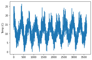
We’ll be working with a temperature demo EntitySet that contains one DataFrame, temperatures. The temperatures dataframe contains the minimum daily temperatures that we will be predicting. In total, it has three columns: id, Temp, and Date. The id column is the index that is necessary for Featuretools’ purposes. The other two are important for univariate time series problems: Date is our time index, and Temp is our target column. The engineered features will be
built from these two columns.
[2]:
es = load_weather()

es['temperatures'].head(10)
Downloading data ...
[2]:
| id | Date | Temp | |
|---|---|---|---|
| 0 | 0 | 1981-01-01 | 20.7 |
| 1 | 1 | 1981-01-02 | 17.9 |
| 2 | 2 | 1981-01-03 | 18.8 |
| 3 | 3 | 1981-01-04 | 14.6 |
| 4 | 4 | 1981-01-05 | 15.8 |
| 5 | 5 | 1981-01-06 | 15.8 |
| 6 | 6 | 1981-01-07 | 15.8 |
| 7 | 7 | 1981-01-08 | 17.4 |
| 8 | 8 | 1981-01-09 | 21.8 |
| 9 | 9 | 1981-01-10 | 20.0 |
[3]:
es['temperatures']['Temp'].plot(ylabel='Temp (C)')
Matplotlib is building the font cache; this may take a moment.
[3]:
<AxesSubplot:ylabel='Temp (C)'>
Understanding The Feature Engineering Window
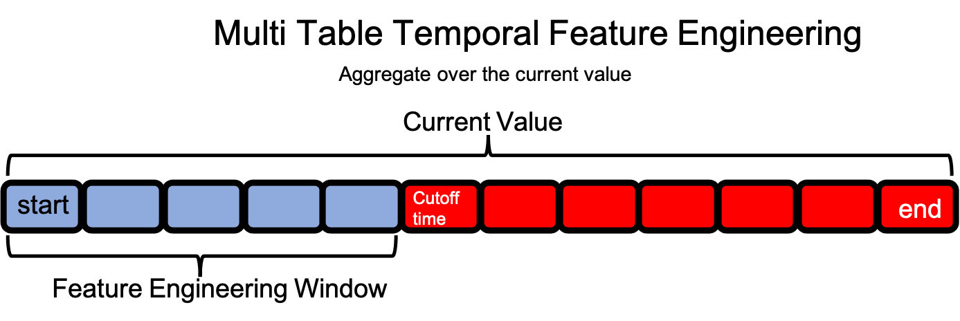
In multi-table datasets, a feature engineering window for a single row in the target DataFrame extends forward in time over observations in child DataFrames starting at the time index and ending when either the cutoff time or last time index is reached.
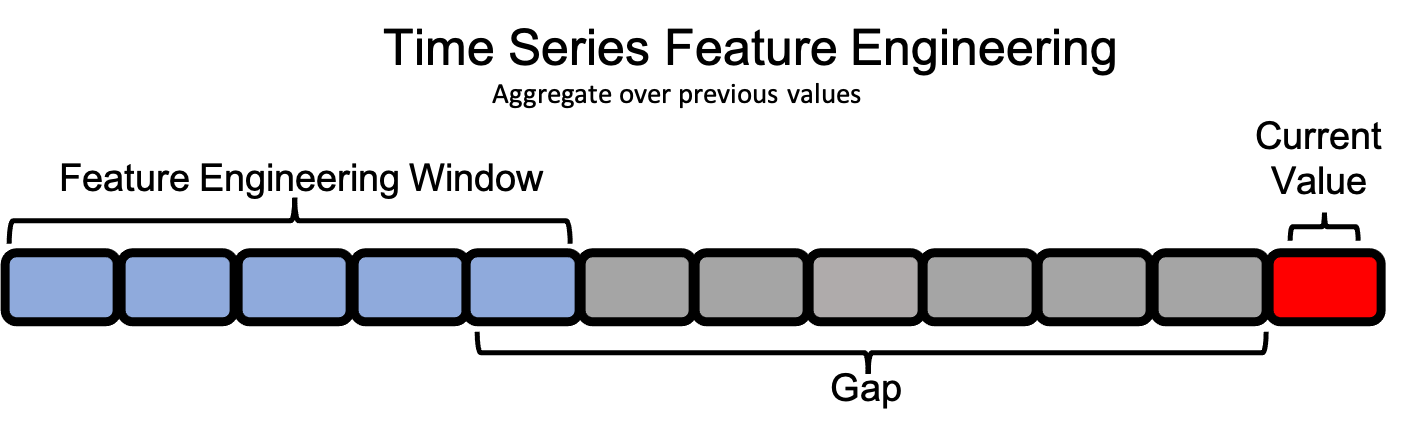
In single-table time series datasets, the feature engineering window for a single value extends backwards in time within the same column. Because of this, the concepts of cutoff time and last time index are not relevant in the same way.
For example: The cutoff time for a single-table time series dataset would create the training and test data split. During DFS, features would not be calculated after the cutoff time. This same behavior can often times be achieved more simply by splitting the data prior to creating the EntitySet, since filtering the data at feature matrix calculation is more computationally intensive than splitting the data ahead of time.
split_point = int(df.shape[0]*.7)

training_data = df[:split_point]
test_data = df[split_point:]
So, since we can’t use the existing parameters for defining each observation’s feature engineering window, we’ll need to define new the concepts of gap and window_length. These will allow us to set a feature engineering window that exists prior to each observation.
Gap and Window Length
Note that we will be using integers when defining the gap and window length. This implies that our data occurs at evenly spaced intervals–in this case daily–so a number n corresponds to n days. Support for unevenly spaced intervals is ongoing and can be explored with the Woodwork method
df.ww.infer_temporal_frequencies.
If we are at a point in time t, we have access to information from times less than t (past values), and we do not have information from times greater than t (future values). Our limitations in feature engineering, then, will come from when exactly before t we have access to the data.
Consider an example where we’re recording data that takes a week to ingest; the earliest data we have access to is from seven days ago, or t - 7. We’ll call this our gap. A gap of 0 would include the instance itself, which we must be careful to avoid in time series problems, as this exposes our target.
We also need to determine how far back in time before t - 7 we can go. Too far back, and we may lose the potency of our recent observations, but too recent, and we may not capture the full spectrum of behaviors displayed by the data. In this example, let’s say that we only want to look at 5 days worth of data at a time. We’ll call this our window_length.
[4]:
gap = 7
window_length = 5
With these two parameters (gap and window_length) set, we have defined our feature engineering window. Now, we can move onto defining our feature primitives.
Time Series Primitives
There are three types of primitives we’ll focus on for time series problems. One of them will extract features from the time index, and the other two types will extract features from our target column.
Datetime Transform Primitives
We need a way of implicating time in our time series features. Yes, using recent temperatures is incredibly predictive in determining future temperatures, but there is also a whole host of historical data suggesting that the month of the year is a pretty good indicator for the temperature outside. However, if we look at the data, we’ll see that, though the day changes, the observations are always taken at the same hour, so the Hour primitive will not likely be useful. Of course, in a dataset
that is measured at an hourly frequency or one more granular, Hour may be incrediby predictive.
[5]:
datetime_primitives = ["Day", "Year", "Weekday", "Month"]
The full list of datetime transform primitives can be seen here.
Delaying Primitives
The simplest thing we can do with our target column is to build features that are delayed (or lagging) versions of the target column. We’ll make one feature per observation in our feature engineering windows, so we’ll range over time from t - gap - window_length to t - gap.
For this purpose, we can use our NumericLag primitive and create one primitive for each instance in our window.
[6]:
delaying_primitives = [NumericLag(periods=i + gap) for i in range(window_length)]
Rolling Transform Primitives
Since we have access to the entire feature engineering window, we can aggregate over that window. Featuretools has several rolling primitives with which we can achieve this. Here, we’ll use the RollingMean and RollingMin primitives, setting the gap and window_length accordingly. Here, the gap is incredibly important, because when the gap is zero, it means the current observation’s taret value is present in the window, which exposes our target.
This concern also exists for other primitives that reference earlier values in the dataframe. Because of this, when using primitives for time series feature engineering, one must be incredibly careful to not use primitives on the target column that incorporate the current observation when calculating a feature value.
[7]:
rolling_mean_primitive = RollingMean(window_length=window_length,
                                     gap=gap,
                                     min_periods=window_length)

rolling_min_primitive = RollingMin(window_length=window_length,
                                     gap=gap,
                                     min_periods=window_length)
The full list of rolling transform primitives can be seen here.
Run DFS
Now that we’ve definied our time series primitives, we can pass them into DFS and get our feature matrix!
Let’s take a look at an actual feature engineering window as we defined with gap and window_length above. Below is an example of how we can extract many features using the same feature engineering window without exposing our target value.
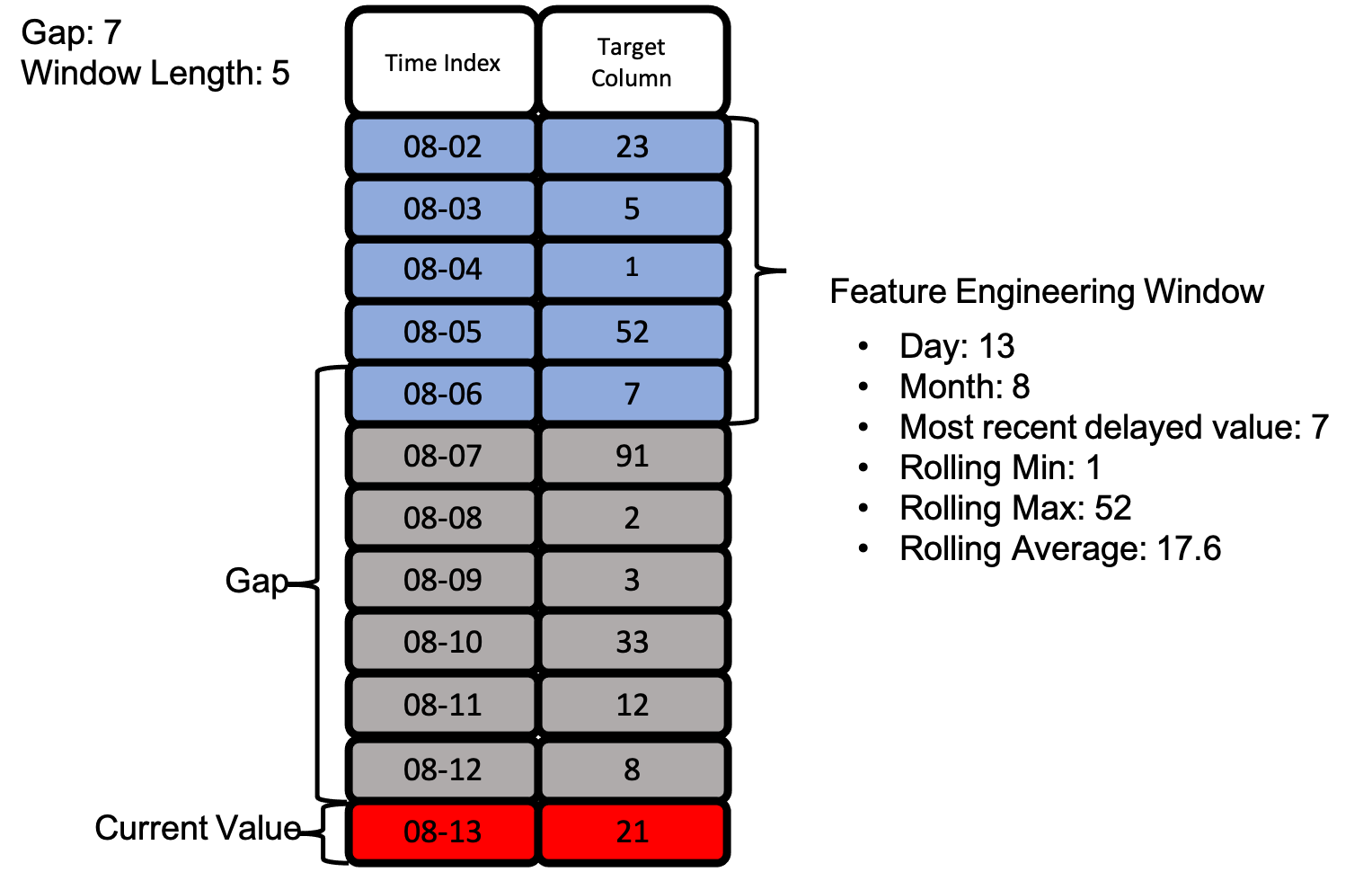
With the image above, we see how all of our defined primitives get used to create many features from just the two columns we have access to.
[8]:
fm, f = ft.dfs(entityset=es,
               target_dataframe_name='temperatures',
               trans_primitives = (datetime_primitives +
                                   delaying_primitives +
                                  [rolling_mean_primitive, rolling_min_primitive]),
               cutoff_time=pd.Timestamp('1987-1-30')
              )

f
[8]:
[<Feature: Temp>,
 <Feature: DAY(Date)>,
 <Feature: MONTH(Date)>,
 <Feature: NUMERIC_LAG(Date, Temp, periods=10)>,
 <Feature: NUMERIC_LAG(Date, Temp, periods=11)>,
 <Feature: NUMERIC_LAG(Date, Temp, periods=7)>,
 <Feature: NUMERIC_LAG(Date, Temp, periods=8)>,
 <Feature: NUMERIC_LAG(Date, Temp, periods=9)>,
 <Feature: ROLLING_MEAN(Date, Temp, window_length=5, gap=7, min_periods=5)>,
 <Feature: ROLLING_MIN(Date, Temp, window_length=5, gap=7, min_periods=5)>,
 <Feature: WEEKDAY(Date)>,
 <Feature: YEAR(Date)>]
[9]:
fm.iloc[:,[0,2, 6, 7, 8, 9]].head(15)
[9]:
| Temp | MONTH(Date) | NUMERIC_LAG(Date, Temp, periods=8) | NUMERIC_LAG(Date, Temp, periods=9) | ROLLING_MEAN(Date, Temp, window_length=5, gap=7, min_periods=5) | ROLLING_MIN(Date, Temp, window_length=5, gap=7, min_periods=5) | |
|---|---|---|---|---|---|---|
| id | ||||||
| 0 | 20.7 | 1 | NaN | NaN | NaN | NaN |
| 1 | 17.9 | 1 | NaN | NaN | NaN | NaN |
| 2 | 18.8 | 1 | NaN | NaN | NaN | NaN |
| 3 | 14.6 | 1 | NaN | NaN | NaN | NaN |
| 4 | 15.8 | 1 | NaN | NaN | NaN | NaN |
| 5 | 15.8 | 1 | NaN | NaN | NaN | NaN |
| 6 | 15.8 | 1 | NaN | NaN | NaN | NaN |
| 7 | 17.4 | 1 | NaN | NaN | NaN | NaN |
| 8 | 21.8 | 1 | 20.7 | NaN | NaN | NaN |
| 9 | 20.0 | 1 | 17.9 | 20.7 | NaN | NaN |
| 10 | 16.2 | 1 | 18.8 | 17.9 | NaN | NaN |
| 11 | 13.3 | 1 | 14.6 | 18.8 | 17.56 | 14.6 |
| 12 | 16.7 | 1 | 15.8 | 14.6 | 16.58 | 14.6 |
| 13 | 21.5 | 1 | 15.8 | 15.8 | 16.16 | 14.6 |
| 14 | 25.0 | 1 | 15.8 | 15.8 | 15.88 | 14.6 |
Above is our time series feature matrix! The rolling and delayed features are built from our target column, but do not expose it. We can now use the feature matrix to create a machine learning model that predicts future minimum daily temperatures.