Handling Time
When performing feature engineering with temporal data, carefully selecting the data that is used for any calculation is paramount. By annotating entities with a time index column and providing a cutoff time during feature calculation, Featuretools will automatically filter out any data after the cutoff time before running any calculations.
What is the Time Index?
The time index is the column in the data that specifies when the data in each row became known. For example, let’s examine a table of customer transactions:
In [1]: import featuretools as ft

In [2]: es = ft.demo.load_mock_customer(return_entityset=True, random_seed=0)

In [3]: es['transactions'].df.head()
Out[3]:
     transaction_id  session_id    transaction_time  amount product_id
298             298           1 2014-01-01 00:00:00  127.64          5
2                 2           1 2014-01-01 00:01:05  109.48          2
308             308           1 2014-01-01 00:02:10   95.06          3
116             116           1 2014-01-01 00:03:15   78.92          4
371             371           1 2014-01-01 00:04:20   31.54          3
In this table, there is one row for every transaction and a transaction_time column that specifies when the transaction took place. This means that transaction_time is the time index because it indicates when the information in each row became known and available for feature calculations.
However, not every datetime column is a time index. Consider the customers entity:
In [4]: es['customers'].df
Out[4]:
   customer_id           join_date date_of_birth zip_code
5            5 2010-07-17 05:27:50    1984-07-28    60091
4            4 2011-04-08 20:08:14    2006-08-15    60091
1            1 2011-04-17 10:48:33    1994-07-18    60091
3            3 2011-08-13 15:42:34    2003-11-21    13244
2            2 2012-04-15 23:31:04    1986-08-18    13244
Here, we have two time columns, join_date and date_of_birth. While either column might be useful for making features, the join_date should be used as the time index because it indicates when that customer first became available in the dataset.
Important
The time index is defined as the first time that any information from a row can be used. If a cutoff time is specified when calculating features, rows that have a later value for the time index are automatically ignored.
What is the Cutoff Time?
The cutoff_time specifies the last point in time that a row’s data can be used for a feature calculation. Any data after this point in time will be filtered out before calculating features.
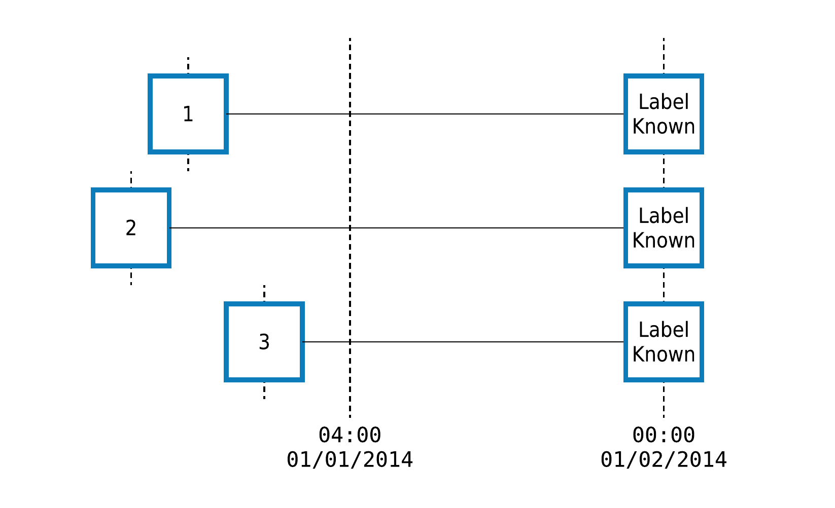
For example, let’s consider a dataset of timestamped customer transactions, where we want to predict whether customers 1, 2 and 3 will spend $500 between 04:00 on January 1 and the end of the day. When building features for this prediction problem, we need to ensure that no data after 04:00 is used in our calculations.
We pass the cutoff time to featuretools.dfs() or featuretools.calculate_feature_matrix() using the cutoff_time argument like this:
In [5]: fm, features = ft.dfs(entityset=es,
...: target_entity='customers',
...: cutoff_time=pd.Timestamp("2014-1-1 04:00"),
...: instance_ids=[1,2,3],
...: cutoff_time_in_index=True)
...:
In [6]: fm
Out[6]:
zip_code COUNT(sessions) NUM_UNIQUE(sessions.device) MODE(sessions.device) SUM(transactions.amount) STD(transactions.amount) MAX(transactions.amount) SKEW(transactions.amount) MIN(transactions.amount) MEAN(transactions.amount) COUNT(transactions) NUM_UNIQUE(transactions.product_id) MODE(transactions.product_id) DAY(date_of_birth) DAY(join_date) YEAR(date_of_birth) YEAR(join_date) MONTH(date_of_birth) MONTH(join_date) WEEKDAY(date_of_birth) WEEKDAY(join_date) SUM(sessions.MAX(transactions.amount)) SUM(sessions.SKEW(transactions.amount)) SUM(sessions.MIN(transactions.amount)) SUM(sessions.NUM_UNIQUE(transactions.product_id)) SUM(sessions.MEAN(transactions.amount)) SUM(sessions.STD(transactions.amount)) STD(sessions.COUNT(transactions)) STD(sessions.MAX(transactions.amount)) STD(sessions.SKEW(transactions.amount)) STD(sessions.MIN(transactions.amount)) STD(sessions.SUM(transactions.amount)) STD(sessions.NUM_UNIQUE(transactions.product_id)) STD(sessions.MEAN(transactions.amount)) MAX(sessions.COUNT(transactions)) MAX(sessions.SKEW(transactions.amount)) MAX(sessions.MIN(transactions.amount)) MAX(sessions.SUM(transactions.amount)) MAX(sessions.NUM_UNIQUE(transactions.product_id)) MAX(sessions.MEAN(transactions.amount)) MAX(sessions.STD(transactions.amount)) SKEW(sessions.COUNT(transactions)) SKEW(sessions.MAX(transactions.amount)) SKEW(sessions.MIN(transactions.amount)) SKEW(sessions.SUM(transactions.amount)) SKEW(sessions.NUM_UNIQUE(transactions.product_id)) SKEW(sessions.MEAN(transactions.amount)) SKEW(sessions.STD(transactions.amount)) MIN(sessions.COUNT(transactions)) MIN(sessions.MAX(transactions.amount)) MIN(sessions.SKEW(transactions.amount)) MIN(sessions.SUM(transactions.amount)) MIN(sessions.NUM_UNIQUE(transactions.product_id)) MIN(sessions.MEAN(transactions.amount)) MIN(sessions.STD(transactions.amount)) MEAN(sessions.COUNT(transactions)) MEAN(sessions.MAX(transactions.amount)) MEAN(sessions.SKEW(transactions.amount)) MEAN(sessions.MIN(transactions.amount)) MEAN(sessions.SUM(transactions.amount)) MEAN(sessions.NUM_UNIQUE(transactions.product_id)) MEAN(sessions.MEAN(transactions.amount)) MEAN(sessions.STD(transactions.amount)) NUM_UNIQUE(sessions.MODE(transactions.product_id)) NUM_UNIQUE(sessions.MONTH(session_start)) NUM_UNIQUE(sessions.YEAR(session_start)) NUM_UNIQUE(sessions.WEEKDAY(session_start)) NUM_UNIQUE(sessions.DAY(session_start)) MODE(sessions.MODE(transactions.product_id)) MODE(sessions.MONTH(session_start)) MODE(sessions.YEAR(session_start)) MODE(sessions.WEEKDAY(session_start)) MODE(sessions.DAY(session_start)) NUM_UNIQUE(transactions.sessions.customer_id) NUM_UNIQUE(transactions.sessions.device) MODE(transactions.sessions.customer_id) MODE(transactions.sessions.device)
customer_id time
1 2014-01-01 04:00:00 60091 4 3 tablet 4958.19 42.309717 139.23 -0.006928 5.81 74.002836 67 5 4 18 17 1994 2011 7 4 0 6 540.04 -0.505043 27.62 20 304.601700 169.572874 5.678908 5.027226 0.500353 1.285833 271.917637 0.0 10.426572 25 0.234349 8.74 1613.93 5 85.469167 46.905665 1.614843 -0.451371 1.452325 1.197406 0.0 -0.233453 1.235445 12 129.00 -0.830975 1025.63 5 64.557200 39.825249 16.75 135.0100 -0.126261 6.905 1239.5475 5 76.150425 42.393218 3 1 1 1 1 4 1 2014 2 1 1 3 1 tablet
2 2014-01-01 04:00:00 13244 4 2 desktop 4150.30 39.289512 146.81 -0.134786 12.07 84.700000 49 5 4 18 15 1986 2012 8 4 0 6 569.29 0.045171 105.24 20 340.791792 157.262738 3.862210 3.470527 0.324809 20.424007 307.743859 0.0 8.983533 16 0.295458 56.46 1320.64 5 96.581000 47.935920 -0.169238 0.459305 1.815491 -0.823347 0.0 0.651941 -0.966834 8 138.38 -0.455197 634.84 5 76.813125 27.839228 12.25 142.3225 0.011293 26.310 1037.5750 5 85.197948 39.315685 3 1 1 1 1 2 1 2014 2 1 1 2 2 desktop
3 2014-01-01 04:00:00 13244 1 1 tablet 941.87 47.264797 146.31 0.618455 8.19 62.791333 15 5 1 21 13 2003 2011 11 8 4 5 146.31 0.618455 8.19 5 62.791333 47.264797 NaN NaN NaN NaN NaN NaN NaN 15 0.618455 8.19 941.87 5 62.791333 47.264797 NaN NaN NaN NaN NaN NaN NaN 15 146.31 0.618455 941.87 5 62.791333 47.264797 15.00 146.3100 0.618455 8.190 941.8700 5 62.791333 47.264797 1 1 1 1 1 1 1 2014 2 1 1 1 3 tablet
Even though the entityset contains the complete transaction history for each customer, only data with a time index up to and including the cutoff time was used to calculate the features above.
Using a Cutoff Time DataFrame
Oftentimes, the training examples for machine learning will come from different points in time. To specify a unique cutoff time for each row of the resulting feature matrix, we can pass a dataframe where the first column is the instance id and the second column is the corresponding cutoff time.
Note
Only the first two columns are used to calculate features. Any additional columns passed through are appended to the resulting feature matrix. This is typically used to pass through machine learning labels to ensure that they stay aligned with the feature matrix.
In [7]: cutoff_times = pd.DataFrame()
In [8]: cutoff_times['customer_id'] = [1, 2, 3, 1]
In [9]: cutoff_times['time'] = pd.to_datetime(['2014-1-1 04:00',
...: '2014-1-1 05:00',
...: '2014-1-1 06:00',
...: '2014-1-1 08:00'])
...:
In [10]: cutoff_times['label'] = [True, True, False, True]
In [11]: cutoff_times
Out[11]:
customer_id time label
0 1 2014-01-01 04:00:00 True
1 2 2014-01-01 05:00:00 True
2 3 2014-01-01 06:00:00 False
3 1 2014-01-01 08:00:00 True
In [12]: fm, features = ft.dfs(entityset=es,
....: target_entity='customers',
....: cutoff_time=cutoff_times,
....: cutoff_time_in_index=True)
....:
In [13]: fm
Out[13]:
zip_code COUNT(sessions) NUM_UNIQUE(sessions.device) MODE(sessions.device) SUM(transactions.amount) STD(transactions.amount) MAX(transactions.amount) SKEW(transactions.amount) MIN(transactions.amount) MEAN(transactions.amount) COUNT(transactions) NUM_UNIQUE(transactions.product_id) MODE(transactions.product_id) DAY(date_of_birth) DAY(join_date) YEAR(date_of_birth) YEAR(join_date) MONTH(date_of_birth) MONTH(join_date) WEEKDAY(date_of_birth) WEEKDAY(join_date) SUM(sessions.MAX(transactions.amount)) SUM(sessions.SKEW(transactions.amount)) SUM(sessions.MIN(transactions.amount)) SUM(sessions.NUM_UNIQUE(transactions.product_id)) SUM(sessions.MEAN(transactions.amount)) SUM(sessions.STD(transactions.amount)) STD(sessions.COUNT(transactions)) STD(sessions.MAX(transactions.amount)) STD(sessions.SKEW(transactions.amount)) STD(sessions.MIN(transactions.amount)) STD(sessions.SUM(transactions.amount)) STD(sessions.NUM_UNIQUE(transactions.product_id)) STD(sessions.MEAN(transactions.amount)) MAX(sessions.COUNT(transactions)) MAX(sessions.SKEW(transactions.amount)) MAX(sessions.MIN(transactions.amount)) MAX(sessions.SUM(transactions.amount)) MAX(sessions.NUM_UNIQUE(transactions.product_id)) MAX(sessions.MEAN(transactions.amount)) MAX(sessions.STD(transactions.amount)) SKEW(sessions.COUNT(transactions)) SKEW(sessions.MAX(transactions.amount)) SKEW(sessions.MIN(transactions.amount)) SKEW(sessions.SUM(transactions.amount)) SKEW(sessions.NUM_UNIQUE(transactions.product_id)) SKEW(sessions.MEAN(transactions.amount)) SKEW(sessions.STD(transactions.amount)) MIN(sessions.COUNT(transactions)) MIN(sessions.MAX(transactions.amount)) MIN(sessions.SKEW(transactions.amount)) MIN(sessions.SUM(transactions.amount)) MIN(sessions.NUM_UNIQUE(transactions.product_id)) MIN(sessions.MEAN(transactions.amount)) MIN(sessions.STD(transactions.amount)) MEAN(sessions.COUNT(transactions)) MEAN(sessions.MAX(transactions.amount)) MEAN(sessions.SKEW(transactions.amount)) MEAN(sessions.MIN(transactions.amount)) MEAN(sessions.SUM(transactions.amount)) MEAN(sessions.NUM_UNIQUE(transactions.product_id)) MEAN(sessions.MEAN(transactions.amount)) MEAN(sessions.STD(transactions.amount)) NUM_UNIQUE(sessions.MODE(transactions.product_id)) NUM_UNIQUE(sessions.MONTH(session_start)) NUM_UNIQUE(sessions.YEAR(session_start)) NUM_UNIQUE(sessions.WEEKDAY(session_start)) NUM_UNIQUE(sessions.DAY(session_start)) MODE(sessions.MODE(transactions.product_id)) MODE(sessions.MONTH(session_start)) MODE(sessions.YEAR(session_start)) MODE(sessions.WEEKDAY(session_start)) MODE(sessions.DAY(session_start)) NUM_UNIQUE(transactions.sessions.customer_id) NUM_UNIQUE(transactions.sessions.device) MODE(transactions.sessions.customer_id) MODE(transactions.sessions.device) label
customer_id time
1 2014-01-01 04:00:00 60091 4 3 tablet 4958.19 42.309717 139.23 -0.006928 5.81 74.002836 67 5 4 18 17 1994 2011 7 4 0 6 540.04 -0.505043 27.62 20 304.601700 169.572874 5.678908 5.027226 0.500353 1.285833 271.917637 0.0 10.426572 25 0.234349 8.74 1613.93 5 85.469167 46.905665 1.614843 -0.451371 1.452325 1.197406 0.0 -0.233453 1.235445 12 129.00 -0.830975 1025.63 5 64.557200 39.825249 16.75 135.01000 -0.126261 6.90500 1239.5475 5 76.150425 42.393218 3 1 1 1 1 4 1 2014 2 1 1 3 1 tablet True
2 2014-01-01 05:00:00 13244 5 2 desktop 5155.26 38.047944 146.81 -0.121811 12.07 83.149355 62 5 4 18 15 1986 2012 8 4 0 6 688.14 -0.269747 127.06 25 418.096407 190.987775 3.361547 10.919023 0.316873 17.801322 266.912832 0.0 8.543351 16 0.295458 56.46 1320.64 5 96.581000 47.935920 -0.379092 -1.814717 1.959531 -0.667256 0.0 1.082192 -0.213518 8 118.85 -0.455197 634.84 5 76.813125 27.839228 12.40 137.62800 -0.053949 25.41200 1031.0520 5 83.619281 38.197555 4 1 1 1 1 2 1 2014 2 1 1 2 2 desktop True
3 2014-01-01 06:00:00 13244 4 2 desktop 2867.69 40.349758 146.31 0.318315 6.65 65.174773 44 5 1 21 13 2003 2011 11 8 4 5 493.07 0.860577 126.66 16 290.968018 119.136697 7.118052 22.808351 0.500999 40.508892 417.557763 2.0 16.540737 17 0.618455 91.76 944.85 5 91.760000 47.264797 -1.330938 -1.060639 1.874170 -1.977878 -2.0 0.201588 1.722323 1 91.76 -0.289466 91.76 1 55.579412 35.704680 11.00 123.26750 0.286859 31.66500 716.9225 4 72.742004 39.712232 2 1 1 1 1 1 1 2014 2 1 1 2 3 desktop False
1 2014-01-01 08:00:00 60091 8 3 mobile 9025.62 40.442059 139.43 0.019698 5.81 71.631905 126 5 4 18 17 1994 2011 7 4 0 6 1057.97 -0.476122 78.59 40 582.193117 312.745952 4.062019 7.322191 0.589386 6.954507 279.510713 0.0 13.759314 25 0.640252 26.36 1613.93 5 88.755625 46.905665 1.946018 -0.780493 2.440005 0.778170 0.0 -0.424949 -0.312355 12 118.90 -1.038434 809.97 5 50.623125 30.450261 15.75 132.24625 -0.059515 9.82375 1128.2025 5 72.774140 39.093244 4 1 1 1 1 4 1 2014 2 1 1 3 1 mobile True
We can now see that every row of the feature matrix is calculated at the corresponding time in the cutoff time dataframe. Because we calculate each row at a different time, it is possible to have a repeat customer. In this case, we calculated the feature vector for customer 1 at both 04:00 and 08:00.
Training Window
By default, all data up to and including the cutoff time is used. We can restrict the amount of historical data that is selected for calculations using a “training window.”
Here’s an example of using a two hour training window:
In [14]: window_fm, window_features = ft.dfs(entityset=es,
....: target_entity="customers",
....: cutoff_time=cutoff_times,
....: cutoff_time_in_index=True,
....: training_window="2 hour")
....:
In [15]: window_fm
Out[15]:
zip_code COUNT(sessions) NUM_UNIQUE(sessions.device) MODE(sessions.device) SUM(transactions.amount) STD(transactions.amount) MAX(transactions.amount) SKEW(transactions.amount) MIN(transactions.amount) MEAN(transactions.amount) COUNT(transactions) NUM_UNIQUE(transactions.product_id) MODE(transactions.product_id) DAY(date_of_birth) DAY(join_date) YEAR(date_of_birth) YEAR(join_date) MONTH(date_of_birth) MONTH(join_date) WEEKDAY(date_of_birth) WEEKDAY(join_date) SUM(sessions.MAX(transactions.amount)) SUM(sessions.SKEW(transactions.amount)) SUM(sessions.MIN(transactions.amount)) SUM(sessions.NUM_UNIQUE(transactions.product_id)) SUM(sessions.MEAN(transactions.amount)) SUM(sessions.STD(transactions.amount)) STD(sessions.COUNT(transactions)) STD(sessions.MAX(transactions.amount)) STD(sessions.SKEW(transactions.amount)) STD(sessions.MIN(transactions.amount)) STD(sessions.SUM(transactions.amount)) STD(sessions.NUM_UNIQUE(transactions.product_id)) STD(sessions.MEAN(transactions.amount)) MAX(sessions.COUNT(transactions)) MAX(sessions.SKEW(transactions.amount)) MAX(sessions.MIN(transactions.amount)) MAX(sessions.SUM(transactions.amount)) MAX(sessions.NUM_UNIQUE(transactions.product_id)) MAX(sessions.MEAN(transactions.amount)) MAX(sessions.STD(transactions.amount)) SKEW(sessions.COUNT(transactions)) SKEW(sessions.MAX(transactions.amount)) SKEW(sessions.MIN(transactions.amount)) SKEW(sessions.SUM(transactions.amount)) SKEW(sessions.NUM_UNIQUE(transactions.product_id)) SKEW(sessions.MEAN(transactions.amount)) SKEW(sessions.STD(transactions.amount)) MIN(sessions.COUNT(transactions)) MIN(sessions.MAX(transactions.amount)) MIN(sessions.SKEW(transactions.amount)) MIN(sessions.SUM(transactions.amount)) MIN(sessions.NUM_UNIQUE(transactions.product_id)) MIN(sessions.MEAN(transactions.amount)) MIN(sessions.STD(transactions.amount)) MEAN(sessions.COUNT(transactions)) MEAN(sessions.MAX(transactions.amount)) MEAN(sessions.SKEW(transactions.amount)) MEAN(sessions.MIN(transactions.amount)) MEAN(sessions.SUM(transactions.amount)) MEAN(sessions.NUM_UNIQUE(transactions.product_id)) MEAN(sessions.MEAN(transactions.amount)) MEAN(sessions.STD(transactions.amount)) NUM_UNIQUE(sessions.MODE(transactions.product_id)) NUM_UNIQUE(sessions.MONTH(session_start)) NUM_UNIQUE(sessions.YEAR(session_start)) NUM_UNIQUE(sessions.WEEKDAY(session_start)) NUM_UNIQUE(sessions.DAY(session_start)) MODE(sessions.MODE(transactions.product_id)) MODE(sessions.MONTH(session_start)) MODE(sessions.YEAR(session_start)) MODE(sessions.WEEKDAY(session_start)) MODE(sessions.DAY(session_start)) NUM_UNIQUE(transactions.sessions.customer_id) NUM_UNIQUE(transactions.sessions.device) MODE(transactions.sessions.customer_id) MODE(transactions.sessions.device) label
customer_id time
1 2014-01-01 04:00:00 60091 2 2 desktop 2077.66 43.772157 139.09 -0.187686 5.81 76.950370 27 5 4 18 17 1994 2011 7 4 0 6 271.81 -0.604638 12.59 10 155.604500 86.730914 2.121320 4.504270 0.747633 0.685894 18.667619 0.000000 10.842658 15 0.226337 6.78 1052.03 5 85.469167 46.905665 NaN NaN NaN NaN NaN NaN NaN 12 132.72 -0.830975 1025.63 5 70.135333 39.825249 13.500000 135.905000 -0.302319 6.295000 1038.830000 5.000000 77.802250 43.365457 2 1 1 1 1 1 1 2014 2 1 1 2 1 desktop True
2 2014-01-01 05:00:00 13244 3 2 desktop 2605.61 36.077146 146.81 -0.198611 12.07 84.051935 31 5 4 18 15 1986 2012 8 4 0 6 404.04 -0.110009 90.35 15 253.240615 109.500185 2.516611 14.342521 0.242542 23.329038 203.331699 0.000000 10.587085 13 0.130019 56.46 1004.96 5 96.581000 47.935920 0.585583 -1.083626 1.397956 -1.660092 0.000000 1.659252 1.121470 8 118.85 -0.314918 634.84 5 77.304615 27.839228 10.333333 134.680000 -0.036670 30.116667 868.536667 5.000000 84.413538 36.500062 3 1 1 1 1 1 1 2014 2 1 1 2 2 desktop True
3 2014-01-01 06:00:00 13244 3 1 desktop 1925.82 37.130891 128.26 0.110145 6.65 66.407586 29 5 1 21 13 2003 2011 11 8 4 5 346.76 0.242122 118.47 11 228.176684 71.871900 8.082904 20.648490 0.580573 45.761028 477.281339 2.309401 18.557570 17 0.531588 91.76 944.85 5 91.760000 36.167220 -0.722109 -1.721498 1.566223 -1.705607 -1.732051 -1.081879 NaN 1 91.76 -0.289466 91.76 1 55.579412 35.704680 9.666667 115.586667 0.121061 39.490000 641.940000 3.666667 76.058895 35.935950 2 1 1 1 1 1 1 2014 2 1 1 1 3 desktop False
1 2014-01-01 08:00:00 60091 3 2 mobile 3124.15 38.952172 139.43 0.047120 5.91 66.471277 47 5 4 18 17 1994 2011 7 4 0 6 384.44 -0.003438 24.61 15 198.984750 107.128899 0.577350 10.415432 0.906666 3.016195 330.655558 0.000000 19.935229 16 0.640252 11.62 1420.09 5 88.755625 44.354104 -1.732051 0.846298 1.443486 1.606791 0.000000 1.344879 1.612576 15 118.90 -1.038434 809.97 5 50.623125 30.450261 15.666667 128.146667 -0.001146 8.203333 1041.383333 5.000000 66.328250 35.709633 3 1 1 1 1 1 1 2014 2 1 1 2 1 mobile True
We can see that that the counts for the same feature are lower after we shorten the training window:
In [16]: fm[["COUNT(transactions)"]]
Out[16]:
                                 COUNT(transactions)
customer_id time
1           2014-01-01 04:00:00                   67
2           2014-01-01 05:00:00                   62
3           2014-01-01 06:00:00                   44
1           2014-01-01 08:00:00                  126

In [17]: window_fm[["COUNT(transactions)"]]
Out[17]:
                                 COUNT(transactions)
customer_id time
1           2014-01-01 04:00:00                   27
2           2014-01-01 05:00:00                   31
3           2014-01-01 06:00:00                   29
1           2014-01-01 08:00:00                   47
Setting a Last Time Index
The training window in Featuretools limits the amount of past data that can be used while calculating a particular feature vector. A row in the entity is filtered out if the value of its time index is either before or after the training window. This works for entities where a row occurs at a single point in time. However, a row can sometimes exist for a duration.
For example, a customer’s session has multiple transactions which can happen at different points in time. If we are trying to count the number of sessions a user has in a given time period, we often want to count all the sessions that had any transaction during the training window. To accomplish this, we need to not only know when a session starts, but also when it ends. The last time that an instance appears in the data is stored as the last_time_index of an Entity. We can compare the time index and the last time index of the sessions entity above:
In [18]: es['sessions'].df['session_start'].head()
Out[18]:
1   2014-01-01 00:00:00
2   2014-01-01 00:17:20
3   2014-01-01 00:28:10
4   2014-01-01 00:44:25
5   2014-01-01 01:11:30
Name: session_start, dtype: datetime64[ns]

In [19]: es['sessions'].last_time_index.head()
Out[19]:
1   2014-01-01 00:16:15
2   2014-01-01 00:27:05
3   2014-01-01 00:43:20
4   2014-01-01 01:10:25
5   2014-01-01 01:22:20
Name: last_time, dtype: datetime64[ns]
Featuretools can automatically add last time indexes to every Entity in an Entityset by running EntitySet.add_last_time_indexes(). If a last_time_index has been set, Featuretools will check to see if the last_time_index is after the start of the training window. That, combined with the cutoff time, allows DFS to discover which data is relevant for a given training window.
Approximating Features by Rounding Cutoff Times
For each unique cutoff time, Featuretools must perform operations to select the data that’s valid for computations. If there are a large number of unique cutoff times relative to the number of instances for which we are calculating features, the time spent filtering data can add up. By reducing the number of unique cutoff times, we minimize the overhead from searching for and extracting data for feature calculations.
One way to decrease the number of unique cutoff times is to round cutoff times to an earlier point in time. An earlier cutoff time is always valid for predictive modeling — it just means we’re not using some of the data we could potentially use while calculating that feature. So, we gain computational speed by losing a small amount of information.
To understand when an approximation is useful, consider calculating features for a model to predict fraudulent credit card transactions. In this case, an important feature might be, “the average transaction amount for this card in the past”. While this value can change every time there is a new transaction, updating it less frequently might not impact accuracy.
Note
The bank BBVA used approximation when building a predictive model for credit card fraud using Featuretools. For more details, see the “Real-time deployment considerations” section of the white paper describing the work involved.
The frequency of approximation is controlled using the approximate parameter to featuretools.dfs() or featuretools.calculate_feature_matrix(). For example, the following code would approximate aggregation features at 1 day intervals:
fm = ft.calculate_feature_matrix(features=features,
                                 entityset=es_transactions,
                                 cutoff_time=ct_transactions,
                                 approximate="1 day")
In this computation, features that can be approximated will be calculated at 1 day intervals, while features that cannot be approximated (e.g “what is the destination of this flight?”) will be calculated at the exact cutoff time.
Secondary Time Index
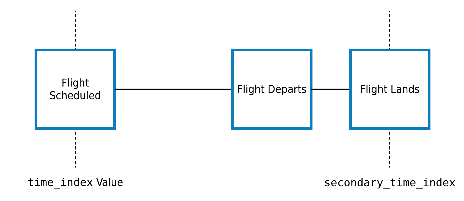
It is sometimes the case that information in a dataset is updated or added after a row has been created. This means that certain columns may actually become known after the time index for a row. Rather than drop those columns to avoid leaking information, we can create a secondary time index to indicate when those columns become known.
The Flights entityset is a good example of a dataset where column values in a row become known at different times. Each trip is recorded in the trip_logs entity, and has many times associated with it.
In [20]: es_flight = ft.demo.load_flight(nrows=100)
Downloading data ...

In [21]: es_flight
Out[21]:
Entityset: Flight Data
  Entities:
    trip_logs [Rows: 100, Columns: 21]
    flights [Rows: 13, Columns: 9]
    airlines [Rows: 1, Columns: 1]
    airports [Rows: 6, Columns: 3]
  Relationships:
    trip_logs.flight_id -> flights.flight_id
    flights.carrier -> airlines.carrier
    flights.dest -> airports.dest

In [22]: es_flight['trip_logs'].df.head(3)
Out[22]:
    trip_log_id        flight_id date_scheduled  scheduled_dep_time  scheduled_arr_time            dep_time            arr_time  dep_delay  taxi_out  taxi_in  arr_delay  scheduled_elapsed_time  air_time  distance  carrier_delay  weather_delay  national_airspace_delay  security_delay  late_aircraft_delay  canceled  diverted
30           30  AA-494:RSW->CLT     2016-09-03 2017-01-01 13:14:00 2017-01-01 15:05:00 2017-01-01 13:03:00 2017-01-01 14:53:00      -11.0      12.0     10.0      -12.0           6660000000000      88.0     600.0            0.0            0.0                      0.0             0.0                  0.0       0.0       0.0
38           38  AA-495:ATL->PHX     2016-09-03 2017-01-01 11:30:00 2017-01-01 15:40:00 2017-01-01 11:24:00 2017-01-01 15:41:00       -6.0      28.0      5.0        1.0          15000000000000     224.0    1587.0            0.0            0.0                      0.0             0.0                  0.0       0.0       0.0
46           46  AA-495:CLT->ATL     2016-09-03 2017-01-01 09:25:00 2017-01-01 10:42:00 2017-01-01 09:23:00 2017-01-01 10:39:00       -2.0      18.0      8.0       -3.0           4620000000000      50.0     226.0            0.0            0.0                      0.0             0.0                  0.0       0.0       0.0
For every trip log, the time index is date_scheduled, which is when the airline decided on the scheduled departure and arrival times, as well as what route will be flown. We don’t know the rest of the information about the actual departure/arrival times and the details of any delay at this time. However, it is possible to know everything about how a trip went after it has arrived, so we can use that information at any time after the flight lands.
Using a secondary time index, we can indicate to Featuretools which columns in our flight logs are known at the time the flight is scheduled, plus which are known at the time the flight lands.
In Featuretools, when creating the entity, we set the secondary time index to be the arrival time like this:
es = ft.EntitySet('Flight Data')
arr_time_columns = ['arr_delay', 'dep_delay', 'carrier_delay', 'weather_delay',
                    'national_airspace_delay', 'security_delay',
                    'late_aircraft_delay', 'canceled', 'diverted',
                    'taxi_in', 'taxi_out', 'air_time', 'dep_time']

es.entity_from_dataframe('trip_logs',
                         data,
                         index='trip_log_id',
                         make_index=True,
                         time_index='date_scheduled',
                         secondary_time_index={'arr_time': arr_time_columns})
By setting a secondary time index, we can still use the delay information from a row, but only when it becomes known.
Hint
It’s often a good idea to use a secondary time index if your entityset has inline labels. If you know when the label would be valid for use, it’s possible to automatically create very predictive features using historical labels.
Flight Predictions
Let’s make some features at varying times using the flight example described above. Trip 14 is a flight from CLT to PHX on January 31, 2017 and trip 92 is a flight from PIT to DFW on January 1. We can set any cutoff time before the flight is scheduled to depart, emulating how we would make the prediction at that point in time.
We set two cutoff times for trip 14 at two different times: one which is more than a month before the flight and another which is only 5 days before. For trip 92, we’ll only set one cutoff time, three days before it is scheduled to leave.

Our cutoff time dataframe looks like this:
In [23]: ct_flight = pd.DataFrame()

In [24]: ct_flight['trip_log_id'] = [14, 14, 92]

In [25]: ct_flight['time'] = pd.to_datetime(['2016-12-28',
   ....:                                     '2017-1-25',
   ....:                                     '2016-12-28'])
   ....:

In [26]: ct_flight['label'] = [True, True, False]

In [27]: ct_flight
Out[27]:
   trip_log_id       time  label
0           14 2016-12-28   True
1           14 2017-01-25   True
2           92 2016-12-28  False
Now, let’s calculate the feature matrix:
In [28]: fm, features = ft.dfs(entityset=es_flight,
   ....:                       target_entity='trip_logs',
   ....:                       cutoff_time=ct_flight,
   ....:                       cutoff_time_in_index=True,
   ....:                       agg_primitives=["max"],
   ....:                       trans_primitives=["month"],)
   ....:

In [29]: fm[['flight_id', 'label', 'flights.MAX(trip_logs.arr_delay)', 'MONTH(scheduled_dep_time)']]
Out[29]:
                              flight_id  label  flights.MAX(trip_logs.arr_delay)  MONTH(scheduled_dep_time)
trip_log_id time
14          2016-12-28  AA-494:CLT->PHX   True                               NaN                          1
            2017-01-25  AA-494:CLT->PHX   True                              33.0                          1
92          2016-12-28  AA-496:PIT->DFW  False                               NaN                          1
Let’s understand the output:
A row was made for every id-time pair in
ct_flight, which is returned as the index of the feature matrix.The output was sorted by cutoff time. Because of the sorting, it’s often helpful to pass in a label with the cutoff time dataframe so that it will remain sorted in the same fashion as the feature matrix. Any additional columns beyond
idandcutoff_timewill not be used for making features.The column
flights.MAX(trip_logs.arr_delay)is not always defined. It can only have any real values when there are historical flights to aggregate. Notice that, for trip14, there wasn’t any historical data when we made the feature a month in advance, but there were flights to aggregate when we shortened it to 5 days. These are powerful features that are often excluded in manual processes because of how hard they are to make.
Creating and Flattening a Feature Tensor
The make_temporal_cutoffs() function generates a series of equally spaced cutoff times from a given set of cutoff times and instance ids.
This function can be paired with DFS to create and flatten a feature tensor rather than making multiple feature matrices at different delays.
The function takes in the the following parameters:
instance_ids (list, pd.Series, or np.ndarray): A list of instances.
cutoffs (list, pd.Series, or np.ndarray): An associated list of cutoff times.
window_size (str or pandas.DateOffset): The amount of time between each cutoff time in the created time series.
start (datetime.datetime or pd.Timestamp): The first cutoff time in the created time series.
num_windows (int): The number of cutoff times to create in the created time series.
Only two of the three options window_size, start, and num_windows need to be specified to uniquely determine an equally-spaced set of cutoff times at which to compute each instance.
If your cutoff times are the ones used above:
In [30]: cutoff_times
Out[30]:
   customer_id                time  label
0            1 2014-01-01 04:00:00   True
1            2 2014-01-01 05:00:00   True
2            3 2014-01-01 06:00:00  False
3            1 2014-01-01 08:00:00   True
Then passing in window_size='1h' and num_windows=2 makes one row an hour over the last two hours to produce the following new dataframe. The result can be directly passed into DFS to make features at the different time points.
In [31]: temporal_cutoffs = ft.make_temporal_cutoffs(cutoff_times['customer_id'],
....: cutoff_times['time'],
....: window_size='1h',
....: num_windows=2)
....:
In [32]: temporal_cutoffs
Out[32]:
time instance_id
0 2014-01-01 03:00:00 1
1 2014-01-01 04:00:00 1
2 2014-01-01 04:00:00 2
3 2014-01-01 05:00:00 2
4 2014-01-01 05:00:00 3
5 2014-01-01 06:00:00 3
6 2014-01-01 07:00:00 1
7 2014-01-01 08:00:00 1
In [33]: fm, features = ft.dfs(entityset=es,
....: target_entity='customers',
....: cutoff_time=temporal_cutoffs,
....: cutoff_time_in_index=True)
....:
In [34]: fm
Out[34]:
zip_code COUNT(sessions) NUM_UNIQUE(sessions.device) MODE(sessions.device) SUM(transactions.amount) STD(transactions.amount) MAX(transactions.amount) SKEW(transactions.amount) MIN(transactions.amount) MEAN(transactions.amount) COUNT(transactions) NUM_UNIQUE(transactions.product_id) MODE(transactions.product_id) DAY(date_of_birth) DAY(join_date) YEAR(date_of_birth) YEAR(join_date) MONTH(date_of_birth) MONTH(join_date) WEEKDAY(date_of_birth) WEEKDAY(join_date) SUM(sessions.MAX(transactions.amount)) SUM(sessions.SKEW(transactions.amount)) SUM(sessions.MIN(transactions.amount)) SUM(sessions.NUM_UNIQUE(transactions.product_id)) SUM(sessions.MEAN(transactions.amount)) SUM(sessions.STD(transactions.amount)) STD(sessions.COUNT(transactions)) STD(sessions.MAX(transactions.amount)) STD(sessions.SKEW(transactions.amount)) STD(sessions.MIN(transactions.amount)) STD(sessions.SUM(transactions.amount)) STD(sessions.NUM_UNIQUE(transactions.product_id)) STD(sessions.MEAN(transactions.amount)) MAX(sessions.COUNT(transactions)) MAX(sessions.SKEW(transactions.amount)) MAX(sessions.MIN(transactions.amount)) MAX(sessions.SUM(transactions.amount)) MAX(sessions.NUM_UNIQUE(transactions.product_id)) MAX(sessions.MEAN(transactions.amount)) MAX(sessions.STD(transactions.amount)) SKEW(sessions.COUNT(transactions)) SKEW(sessions.MAX(transactions.amount)) SKEW(sessions.MIN(transactions.amount)) SKEW(sessions.SUM(transactions.amount)) SKEW(sessions.NUM_UNIQUE(transactions.product_id)) SKEW(sessions.MEAN(transactions.amount)) SKEW(sessions.STD(transactions.amount)) MIN(sessions.COUNT(transactions)) MIN(sessions.MAX(transactions.amount)) MIN(sessions.SKEW(transactions.amount)) MIN(sessions.SUM(transactions.amount)) MIN(sessions.NUM_UNIQUE(transactions.product_id)) MIN(sessions.MEAN(transactions.amount)) MIN(sessions.STD(transactions.amount)) MEAN(sessions.COUNT(transactions)) MEAN(sessions.MAX(transactions.amount)) MEAN(sessions.SKEW(transactions.amount)) MEAN(sessions.MIN(transactions.amount)) MEAN(sessions.SUM(transactions.amount)) MEAN(sessions.NUM_UNIQUE(transactions.product_id)) MEAN(sessions.MEAN(transactions.amount)) MEAN(sessions.STD(transactions.amount)) NUM_UNIQUE(sessions.MODE(transactions.product_id)) NUM_UNIQUE(sessions.MONTH(session_start)) NUM_UNIQUE(sessions.YEAR(session_start)) NUM_UNIQUE(sessions.WEEKDAY(session_start)) NUM_UNIQUE(sessions.DAY(session_start)) MODE(sessions.MODE(transactions.product_id)) MODE(sessions.MONTH(session_start)) MODE(sessions.YEAR(session_start)) MODE(sessions.WEEKDAY(session_start)) MODE(sessions.DAY(session_start)) NUM_UNIQUE(transactions.sessions.customer_id) NUM_UNIQUE(transactions.sessions.device) MODE(transactions.sessions.customer_id) MODE(transactions.sessions.device)
customer_id time
1 2014-01-01 03:00:00 60091 3 3 desktop 3932.56 42.769602 139.23 0.140387 5.81 71.501091 55 5 1 18 17 1994 2011 7 4 0 6 400.95 0.325932 20.84 15 219.132533 129.747625 5.773503 5.178021 0.210827 1.571507 283.551883 0.0 10.255607 25 0.234349 8.74 1613.93 5 84.440000 46.905665 1.732051 0.782152 1.552040 0.685199 0.0 1.173675 0.763052 15 129.00 -0.134754 1052.03 5 64.557200 40.187205 18.333333 133.650000 0.108644 6.946667 1310.853333 5 73.044178 43.249208 3 1 1 1 1 1 1 2014 2 1 1 3 1 mobile
2014-01-01 04:00:00 60091 4 3 tablet 4958.19 42.309717 139.23 -0.006928 5.81 74.002836 67 5 4 18 17 1994 2011 7 4 0 6 540.04 -0.505043 27.62 20 304.601700 169.572874 5.678908 5.027226 0.500353 1.285833 271.917637 0.0 10.426572 25 0.234349 8.74 1613.93 5 85.469167 46.905665 1.614843 -0.451371 1.452325 1.197406 0.0 -0.233453 1.235445 12 129.00 -0.830975 1025.63 5 64.557200 39.825249 16.750000 135.010000 -0.126261 6.905000 1239.547500 5 76.150425 42.393218 3 1 1 1 1 4 1 2014 2 1 1 3 1 tablet
2 2014-01-01 04:00:00 13244 4 2 desktop 4150.30 39.289512 146.81 -0.134786 12.07 84.700000 49 5 4 18 15 1986 2012 8 4 0 6 569.29 0.045171 105.24 20 340.791792 157.262738 3.862210 3.470527 0.324809 20.424007 307.743859 0.0 8.983533 16 0.295458 56.46 1320.64 5 96.581000 47.935920 -0.169238 0.459305 1.815491 -0.823347 0.0 0.651941 -0.966834 8 138.38 -0.455197 634.84 5 76.813125 27.839228 12.250000 142.322500 0.011293 26.310000 1037.575000 5 85.197948 39.315685 3 1 1 1 1 2 1 2014 2 1 1 2 2 desktop
2014-01-01 05:00:00 13244 5 2 desktop 5155.26 38.047944 146.81 -0.121811 12.07 83.149355 62 5 4 18 15 1986 2012 8 4 0 6 688.14 -0.269747 127.06 25 418.096407 190.987775 3.361547 10.919023 0.316873 17.801322 266.912832 0.0 8.543351 16 0.295458 56.46 1320.64 5 96.581000 47.935920 -0.379092 -1.814717 1.959531 -0.667256 0.0 1.082192 -0.213518 8 118.85 -0.455197 634.84 5 76.813125 27.839228 12.400000 137.628000 -0.053949 25.412000 1031.052000 5 83.619281 38.197555 4 1 1 1 1 2 1 2014 2 1 1 2 2 desktop
3 2014-01-01 05:00:00 13244 2 2 desktop 1886.72 41.199361 146.31 0.637074 6.65 58.960000 32 5 1 21 13 2003 2011 11 8 4 5 273.05 1.150043 14.84 10 118.370745 83.432017 1.414214 13.838080 0.061424 1.088944 2.107178 0.0 5.099599 17 0.618455 8.19 944.85 5 62.791333 47.264797 NaN NaN NaN NaN NaN NaN NaN 15 126.74 0.531588 941.87 5 55.579412 36.167220 16.000000 136.525000 0.575022 7.420000 943.360000 5 59.185373 41.716008 1 1 1 1 1 1 1 2014 2 1 1 2 3 desktop
2014-01-01 06:00:00 13244 4 2 desktop 2867.69 40.349758 146.31 0.318315 6.65 65.174773 44 5 1 21 13 2003 2011 11 8 4 5 493.07 0.860577 126.66 16 290.968018 119.136697 7.118052 22.808351 0.500999 40.508892 417.557763 2.0 16.540737 17 0.618455 91.76 944.85 5 91.760000 47.264797 -1.330938 -1.060639 1.874170 -1.977878 -2.0 0.201588 1.722323 1 91.76 -0.289466 91.76 1 55.579412 35.704680 11.000000 123.267500 0.286859 31.665000 716.922500 4 72.742004 39.712232 2 1 1 1 1 1 1 2014 2 1 1 2 3 desktop
1 2014-01-01 07:00:00 60091 7 3 tablet 7605.53 41.018896 139.43 0.149908 5.81 69.141182 110 5 4 18 17 1994 2011 7 4 0 6 931.86 0.562312 66.97 35 493.437492 280.421418 4.386125 7.441648 0.471955 7.470707 273.713405 0.0 13.123365 25 0.640252 26.36 1613.93 5 85.469167 46.905665 1.927658 -1.277394 2.552328 1.377768 0.0 -0.282093 -0.755846 12 118.90 -0.830975 809.97 5 50.623125 30.450261 15.714286 133.122857 0.080330 9.567143 1086.504286 5 70.491070 40.060203 4 1 1 1 1 1 1 2014 2 1 1 3 1 tablet
2014-01-01 08:00:00 60091 8 3 mobile 9025.62 40.442059 139.43 0.019698 5.81 71.631905 126 5 4 18 17 1994 2011 7 4 0 6 1057.97 -0.476122 78.59 40 582.193117 312.745952 4.062019 7.322191 0.589386 6.954507 279.510713 0.0 13.759314 25 0.640252 26.36 1613.93 5 88.755625 46.905665 1.946018 -0.780493 2.440005 0.778170 0.0 -0.424949 -0.312355 12 118.90 -1.038434 809.97 5 50.623125 30.450261 15.750000 132.246250 -0.059515 9.823750 1128.202500 5 72.774140 39.093244 4 1 1 1 1 4 1 2014 2 1 1 3 1 mobile